
Partial differential equation
Did you know...
SOS Children, an education charity, organised this selection. Visit the SOS Children website at http://www.soschildren.org/
In mathematics, partial differential equations (PDE) are a type of differential equation, i.e., a relation involving an unknown function (or functions) of several independent variables and its (resp. their) partial derivatives with respect to those variables. Partial differential equations are used to formulate, and thus aid the solution of, problems involving functions of several variables; such as the propagation of sound or heat, electrostatics, electrodynamics, fluid flow, elasticity. Interestingly, seemingly distinct physical phenomena may have identical mathematical formulations, and thus be governed by the same underlying dynamic.
Introduction
A relatively simple partial differential equation is
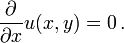
This relation implies that the values u(x,y) are independent of x. Hence the general solution of this equation is
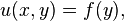
where f is an arbitrary (differentiable) function of y. The analogous ordinary differential equation is

which has the solution

where c is any constant value (independent of x). These two examples illustrate that general solutions of ordinary differential equations involve arbitrary constants, but solutions of partial differential equations involve arbitrary functions. A solution of a partial differential equation is generally not unique; additional conditions must generally be specified on the boundary of the region where the solution is defined. For instance, in the simple example above, the function  can be determined if
  is specified on the line
  .
.
Existence and uniqueness
Although the issue of the existence and uniqueness of solutions of ordinary differential equations has a very satisfactory answer with the Picard-Lindelöf theorem, that is far from the case for partial differential equations. There is a general theorem (the Cauchy-Kovalevskaya theorem) that states that the Cauchy problem for any partial differential equation that is analytic in the unknown function and its derivatives have a unique analytic solution. Although this result might appear to settle the existence and uniqueness of solutions, there are examples of linear partial differential equations whose coefficients have derivatives of all orders (which are nevertheless not analytic) but which have no solutions at all: see Lewy (1957). Even if the solution of a partial differential equation exists and is unique, it may nevertheless have undesirable properties.
An example of pathological behaviour is the sequence of Cauchy problems (depending upon n) for the Laplace equation
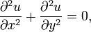
with initial conditions

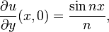
where n is an integer. The derivative of u with respect to y approaches 0 uniformly in x as n increases, but the solution is
This solution approaches infinity if nx is not an integer multiple of π for any non-zero value of y. The Cauchy problem for the Laplace equation is called ill-posed or not well posed, since the solution does not depend continuously upon the data of the problem. Such ill-posed problems are not usually satisfactory for physical applications.
Notation and examples
In PDEs, it is common to denote partial derivatives using subscripts. That is:

Especially in (mathematical) physics, one often prefers use of del (which in cartesian coordinates is written  for spatial derivatives and a dot
  for time derivatives, e.g. to write the wave equation (see below) as
 (math notation)
 (physics notation)
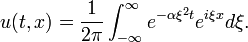
Heat equation in one space dimension
The equation for conduction of heat in one dimension for a homogeneous body has the form

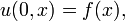
where u(t,x) is temperature, and α is a positive constant that describes the rate of diffusion. The Cauchy problem for this equation consists in specifying 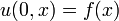 , where f(x) is an arbitrary function.
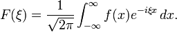
General solutions of the heat equation can be found by the method of separation of variables. Some examples appear in the heat equation article. They are examples of Fourier series for periodic f and Fourier transforms for non-periodic f. Using the Fourier transform, a general solution of the heat equation has the form
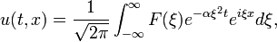
where F is an arbitrary function. In order to satisfy the initial condition, F is given by the Fourier transform of f, that is
If f represents a very small but intense source of heat, then the preceding integral can be approximated by the delta distribution, multiplied by the strength of the source. For a source whose strength is normalized to 1, the result is
and the resulting solution of the heat equation is
This is a Gaussian integral. It may be evaluated to obtain
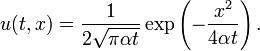
This result corresponds to a normal probability density for x with mean 0 and variance 2αt. The heat equation and similar diffusion equations are useful tools to study random phenomena.
Wave equation in one spatial dimension
The wave equation is an equation for an unknown function u(t, x) of the form

Here u might describe the displacement of a stretched string from equilibrium, or the difference in air pressure in a tube, or the magnitude of an electromagnetic field in a tube, and c is a number that corresponds to the velocity of the wave. The Cauchy problem for this equation consists in prescribing the initial displacement and velocity of a string or other medium:
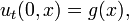
where f and g are arbitrary given functions. The solution of this problem is given by d'Alembert's formula:
![u(t,x) = \frac{1}{2} \left[f(x-ct) + f(x+ct)\right] + \frac{1}{2c}\int_{x-ct}^{x+ct} g(y)\, dy. \,](../../images/89/8985.png)
This formula implies that the solution at (t,x) depends only upon the data on the segment of the initial line that is cut out by the characteristic curves

that are drawn backwards from that point. These curves correspond to signals that propagate with velocity c forward and backward. Conversely, the influence of the data at any given point on the initial line propagates with the finite velocity c: there is no effect outside a triangle through that point whose sides are characteristic curves. This behaviour is very different from the solution for the heat equation, where the effect of a point source appears (with small amplitude) instantaneously at every point in space. The solution given above is also valid if t is negative, and the explicit formula shows that the solution depends smoothly upon the data: both the forward and backward Cauchy problems for the wave equation are well-posed.
Spherical waves
Spherical waves are waves whose amplitude depends only upon the radial distance r from a central point source. For such waves, the three-dimensional wave equation takes the form
![u_{tt} = c^2 \left[u_{rr} + \frac{2}{r} u_r \right]. \,](../../images/89/8987.png)
This is equivalent to
![(ru)_{tt} = c^2 \left[(ru)_{rr} \right],\,](../../images/89/8988.png)
and hence the quantity ru satisfies the one-dimensional wave equation. Therefore a general solution for spherical waves has the form
![u(t,r) = \frac{1}{r} \left[F(r-ct) + G(r+ct) \right],\,](../../images/89/8989.png)
where F and G are completely arbitrary functions. Radiation from an antenna corresponds to the case where G is identically zero. Thus the wave form transmitted from an antenna has no distortion in time: the only distorting factor is 1/r. This feature of undistorted propagation of waves is not present if there are two spatial dimensions.
Laplace equation in two dimensions
The Laplace equation for an unknown function of two variables φ has the form
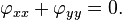
Solutions of Laplace's equation are called harmonic functions.
Connection with functions
Solutions of the Laplace equation are intimately connected with analytic functions of a complex variable (a.k.a. holomorphic functions): the real and imaginary parts of any analytic function are conjugate harmonic functions: they both satisfy the Laplace equation, and their gradients are orthogonal. If f=u+iv, then the Cauchy-Riemann equations state that

and it follows that

Conversely, given any harmonic function, it is the real part of an analytic function, at least locally. Details are given in Laplace equation.
A typical boundary value problem
A typical problem for Laplace's equation is to find a solution that satisfies arbitrary values on the boundary of a domain. For example, we may seek a harmonic function that takes on the values u(θ) on a circle of radius one. The solution was given by Poisson:
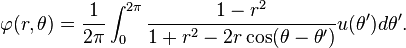
Petrovsky (1967, p. 248) shows how this formula can be obtained by summing a Fourier series for φ. If r<1, the derivatives of φ may be computed by differentiating under the integral sign, and one can verify that φ is analytic, even if u is continuous but not necessarily differentiable. This behaviour is typical for solutions of elliptic partial differential equations: the solutions may be much more smooth than the boundary data. This is in contrast to solutions of the wave equation, and more general hyperbolic partial differential equations, which typically have no more derivatives than the data.
Euler-Tricomi equation
The Euler-Tricomi equation is used in the investigation of transonic flow. It is
Advection equation
The advection equation describes the transport of a conserved scalar  in a velocity field
  . It is:

If the velocity field is solenoidal (that is,  ), then the equation may be simplified to

The one dimensional steady flow advection equation 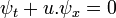 (where is constant) is commonly referred to as the pigpen problem. If is not constant and equal to the equation is referred to as Burgers' equation.
Ginzburg-Landau equation
The Ginzburg-Landau equation is used in modelling superconductivity. It is

where  and
and  are constants and
  is the imaginary unit.
The Dym equation
The Dym equation is named for Harry Dym and occurs in the study of solitons. It is

Other examples
The Schrödinger equation is a PDE at the heart of non-relativistic quantum mechanics. In the WKB approximation it is the Hamilton-Jacobi equation.
Except for the Dym equation and the Ginzburg-Landau equation, the above equations are linear in the sense that they can be written in the form Au = f for a given linear operator A and a given function f. Other important non-linear equations include the Navier-Stokes equations describing the flow of fluids, and Einstein's field equations of general relativity.
Methods to solve PDEs
The method of separation of variables will yield particular solutions of a linear PDE on very simple domains such as rectangles that may satisfy initial or boundary conditions. Because any superposition of solutions of a linear PDE is again a solution, the particular solutions may then be combined to obtain more general solutions. If the domain is finite or periodic, an infinite sum of solutions such as a Fourier series is appropriate, but an integral of solutions such as a Fourier integral is generally required for infinite domains. The solution for a point source for the heat equation given above is an example for use of a Fourier integral.
Initial-boundary value problems
Many problems of Mathematical Physics are formulated as initial-boundary value problems.
Vibrating string
If the string is stretched between two points where x=0 and x=L and u denotes the amplitude of the displacement of the string, then u satisfies the one-dimensional wave equation in the region where 0<x<L and t is unlimited. Since the string is tied down at the ends, u must also satisfy the boundary conditions

as well as the initial conditions

The method of separation of variables for the wave equation

leads to solutions of the form

where

where the constant k must be determined. The boundary conditions then imply that X is a multiple of sin kx, and k must have the form

where n is an integer. Each term in the sum corresponds to a mode of vibration of the string. The mode with n=1 is called the fundamental mode, and the frequencies of the other modes are all multiples of this frequency. They form the overtone series of the string, and they are the basis for musical acoustics. The initial conditions may then be satisfied by representing f and g as infinite sums of these modes. Wind instruments typically correspond to vibrations of an air column with one end open and one end closed. The corresponding boundary conditions are

The method of separation of variables can also be applied in this case, and it leads to a series of odd overtones.
The general problem of this type is solved in Sturm-Liouville theory.
Vibrating membrane
If a membrane is stretched over a curve C that forms the boundary of a domain D in the plane, its vibrations are governed by the wave equation

if t>0 and (x,y) is in D. The boundary condition is  if
if  is on
is on  . The method of separation of variables leads to the form

which in turn must satisfy


The latter equation is called the Helmholtz Equation. The constant k must be determined in order to allow a non-trivial v to satisfy the boundary condition on C. Such values of k2 are called the eigenvalues of the Laplacian in D, and the associated solutions are the eigenfunctions of the Laplacian in D. The Sturm-Liouville theory may be extended to this elliptic eigenvalue problem (Jost, 2002).
There are no generally applicable methods to solve non-linear PDEs. Still, existence and uniqueness results (such as the Cauchy-Kovalevskaya theorem) are often possible, as are proofs of important qualitative and quantitative properties of solutions (getting these results is a major part of analysis). Computational solution to the nonlinear PDEs, the Split-step method, exist for specific equations like Non-Linear Schrodinger equation.
Nevertheless, some techniques can be used for several types of equations. The h-principle is the most powerful method to solve underdetermined equations. The Riquier-Janet theory is an effective method for obtaining information about many analytic overdetermined systems.
The method of characteristics ( Similarity Transformation method) can be used in some very special cases to solve partial differential equations.
In some cases, a PDE can be solved via perturbation analysis in which the solution is considered to be a correction to an equation with a known solution. Alternatives are numerical analysis techniques from simple finite difference schemes to the more mature multigrid and finite element methods. Many interesting problems in science and engineering are solved in this way using computers, sometimes high performance supercomputers.
Classification
Some linear, second-order partial differential equations can be classified as parabolic, hyperbolic or elliptic. Others such as the Euler-Tricomi equation have different types in different regions. The classification provides a guide to appropriate initial and boundary conditions, and to smoothness of the solutions.
Equations of second order
Assuming  , the general second-order PDE in two independent variables has the form

where the coefficients A, B, C etc. may depend upon x and y. This form is analogous to the equation for a conic section:

Just as one classifies conic sections into parabolic, hyperbolic, and elliptic based on the discriminant  , the same can be done for a second-order PDE at a given point.
 : solutions of elliptic PDEs are as smooth as the coefficients allow, within the interior of the region where the equation and solutions are defined. For example, solutions of Laplace's equation are analytic within the domain where they are defined, but solutions may assume boundary values that are not smooth. The motion of a fluid at subsonic speeds can be approximated with elliptic PDEs, and the Euler-Tricomi equation is elliptic where x<0.
 : equations that are parabolic at every point can be transformed into a form analogous to the heat equation by a change of independent variables. Solutions smooth out as the transformed time variable increases. The Euler-Tricomi equation has parabolic type on the line where x=0.
 : hyperbolic equations retain any discontinuities of functions or derivatives in the initial data. An example is the wave equation. The motion of a fluid at supersonic speeds can be approximated with hyperbolic PDEs, and the Euler-Tricomi equation is hyperbolic where x>0.
If there are n independent variables x1, x2 , ..., xn, a general linear partial differential equation of second order has the form

The classification depends upon the signature of the eigenvalues of the coefficient matrix.
- Elliptic: The eigenvalues are all positive or all negative.
- Parabolic : The eigenvalues are all positive or all negative, save one which is zero.
- Hyperbolic: There is only one negative eigenvalue and all the rest are positive, or there is only one positive eigenvalue and all the rest are negative.
- Ultrahyperbolic: There is more than one positive eigenvalue and more than one negative eigenvalue, and there are no zero eigenvalues. There is only limited theory for ultrahyperbolic equations (Courant and Hilbert, 1962).
Systems of first-order equations and characteristic surfaces
The classification of partial differential equations can be extended to systems of first-order equations, where the unknown u is now a vector with m components, and the coefficient matrices  are m by m matrices for
  . The partial differential equation takes the form

where the coefficient matrices Aν and the vector B may depend upon x and u. If a hypersurface S is given in the implicit form

where φ has a non-zero gradient, then S is a characteristic surface for the operator L at a given point if the characteristic form vanishes:
![Q\left(\frac{\part\varphi}{\partial x_1}, \ldots,\frac{\part\varphi}{\partial x_n}\right) =\det\left[\sum_{\nu=1}^nA_\nu \frac{\partial \varphi}{\partial x_\nu}\right]=0.\,](../../images/90/9030.png)
The geometric interpretation of this condition is as follows: if data for u are prescribed on the surface S, then it may be possible to determine the normal derivative of u on S from the differential equation. If the data on S and the differential equation determine the normal derivative of u on S, then S is non-characteristic. If the data on S and the differential equation do not determine the normal derivative of u on S, then the surface is characteristic, and the differential equation restricts the data on S: the differential equation is internal to S.
- A first-order system Lu=0 is elliptic if no surface is characteristic for L: the values of u on S and the differential equation always determine the normal derivative of u on S.
- A first-order system is hyperbolic at a point if there is a space-like surface S with normal ξ at that point. This means that, given any non-trivial vector η orthogonal to ξ, and a scalar multiplier λ, the equation

has m real roots λ1, λ2, ..., λm. The system is strictly hyperbolic if these roots are always distinct. The geometrical interpretation of this condition is as follows: the characteristic form Q(ζ)=0 defines a cone (the normal cone) with homogeneous coordinates ζ. In the hyperbolic case, this cone has m sheets, and the axis ζ = λ ξ runs inside these sheets: it does not intersect any of them. But when displaced from the origin by η, this axis intersects every sheet. In the elliptic case, the normal cone has no real sheets.
Equations of mixed type
If a PDE has coefficients which are not constant, it is possible that it will not belong to any of these categories but rather be of mixed type. A simple but important example is the Euler-Tricomi equation

which is called elliptic-hyperbolic because it is elliptic in the region x < 0, hyperbolic in the region x > 0, and degenerate parabolic on the line x = 0.