Regression analysis

Related subjects: Mathematics

Background Information

SOS Children has tried to make Wikipedia content more accessible by this schools selection. With SOS Children you can choose to sponsor children in over a hundred countries

Regression analysis is a technique used for the modeling and analysis of numerical data consisting of values of a dependent variable (response variable) and of one or more independent variables (explanatory variables). The dependent variable in the regression equation is modeled as a function of the independent variables, corresponding parameters ("constants"), and an error term. The error term is treated as a random variable. It represents unexplained variation in the dependent variable. The parameters are estimated so as to give a "best fit" of the data. Most commonly the best fit is evaluated by using the least squares method, but other criteria have also been used.

Data modeling can be used without there being any knowledge about the underlying processes that have generated the data; in this case the model is an empirical model. Moreover, in modelling knowledge of the probability distribution of the errors is not required. Regression analysis requires assumptions to be made regarding probability distribution of the errors. Statistical tests are made on the basis of these assumptions. In regression analysis the term "model" embraces both the function used to model the data and the assumptions concerning probability distributions.

Regression can be used for prediction (including forecasting of time-series data), inference, hypothesis testing, and modeling of causal relationships. These uses of regression rely heavily on the underlying assumptions being satisfied. Regression analysis has been criticized as being misused for these purposes in many cases where the appropriate assumptions cannot be verified to hold. One factor contributing to the misuse of regression is that it can take considerably more skill to critique a model than to fit a model.

History of regression analysis

The earliest form of regression was the method of least squares, which was published by Legendre in 1805, and by Gauss in 1809. The term “least squares” is from Legendre’s term, moindres carrés. However, Gauss claimed that he had known the method since 1795.

Legendre and Gauss both applied the method to the problem of determining, from astronomical observations, the orbits of bodies about the sun. Euler had worked on the same problem (1748) without success. Gauss published a further development of the theory of least squares in 1821, including a version of the Gauss–Markov theorem.

The term "regression" was coined in the nineteenth century to describe a biological phenomenon, namely that the progeny of exceptional individuals tend on average to be less exceptional than their parents and more like their more distant ancestors. Francis Galton, a cousin of Charles Darwin, studied this phenomenon and applied the slightly misleading term " regression towards mediocrity" to it. For Galton, regression had only this biological meaning, but his work was later extended by Udny Yule and Karl Pearson to a more general statistical context. Nowadays the term "regression" is often synonymous with "least squares curve fitting".

Underlying assumptions

The sample must be representative of the population for the inference prediction.
The dependent variable is subject to error. This error is assumed to be a random variable, with a mean of zero. Systematic error may be present but its treatment is outside the scope of regression analysis.
The independent variable is error-free. If this is not so, modeling should be done using Errors-in-variables model techniques.
The predictors must be linearly independent, i.e. it must not be possible to express any predictor as a linear combination of the others. See Multicollinear.
The errors are uncorrelated, that is, the variance-covariance matrix of the errors is diagonal and each non-zero element is the variance of the error.
The variance of the error is constant ( homoscedasticity). If not, weights should be used.
The errors follow a normal distribution. If not, the generalized linear model should be used.

Linear regression

In linear regression, the model specification is that the dependent variable, $y_i$ is a linear combination of the parameters (but need not be linear in the independent variables). For example, in simple linear regression there is one independent variable, $x_i$ , and two parameters, $\beta_0$ and $\beta_1$ :

straight line: $y_i=\beta_0 +\beta_1 x_i +\epsilon_i,\ i=1,m\!$

In multiple linear regression, there are several independent variables or functions of independent variables. For example, adding a term in x_i² to the preceding regression gives:

parabola: $y_i=\beta_0 +\beta_1 x_i +\beta_2 x_i^2+\epsilon_i,\ i=1,m\!$

This is still linear regression as although the expression on the right hand side is quadratic in the independent variable $x_i$ , it is linear in the parameters $\beta_0$ , $\beta_1$ and $\beta_2.$

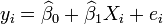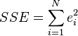
In both cases, $\epsilon_i$ is an error term and the subscript $i$ indexes a particular observation. Given a random sample from the population, we estimate the population parameters and obtain the sample linear regression model: $y_i = \widehat{\beta}_0 + \widehat{\beta}_1 X_i + e_i$ The term $e_i$ is the residual, $e_i = y_i - \widehat{y}_i$ . One method of estimation is Ordinary [Least Squares]. This method obtains parameter estimates that minimize the sum of squared residuals, SSE:

$SSE=\sum_{i=1}^{N}e_i^2$

Minimization of this function results in a set of normal equations, a set of simultaneous linear equations in the parameters, which are solved to yield the parameter estimators, $\widehat{\beta}_0, \widehat{\beta}_1$ . See regression coefficients for statistical properties of these estimators.

Illustration of linear regression on a data set (red points).

In the case of simple regression, the formulas for the least squares estimates are

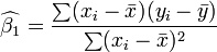$\widehat{\beta_1}=\frac{\sum(x_i-\bar{x})(y_i-\bar{y})}{\sum(x_i-\bar{x})^2}$ and $\hat{\beta_0}=\bar{y}-\hat{\beta}\bar{x}$

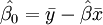
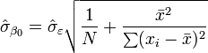
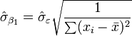
where $\bar{x}$ is the mean (average) of the $x$ values and $\bar{y}$ is the mean of the $y$ values. See linear least squares(straight line fitting) for a derivation of these formulas and a numerical example. Under the assumption that the population error term has a constant variance, the estimate of that variance is given by: 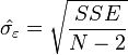$\hat{\sigma_{\varepsilon}} = \sqrt{\frac{SSE}{N-2}}$ This is called the root mean square error (RMSE) of the regression. The standard errors of the parameter estimates are given by

$\hat\sigma_{\beta_0}=\hat\sigma_{\varepsilon} \sqrt{\frac{1}{N} + \frac{\bar{x}^2}{\sum(x_i-\bar x)^2}}$

$\hat\sigma_{\beta_1}=\hat\sigma_{\varepsilon} \sqrt{\frac{1}{\sum(x_i-\bar x)^2}}$

Under the further assumption that the population error term is normally distributed, the researcher can use these estimated standard errors to create confidence intervals and conduct hypothesis tests about the population parameters.

General linear data model

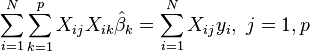
In the more general multiple regression model, there are p independent variables: $y_i = \beta_0 + \beta_1 x_{1i} + \cdots + \beta_p x_{pi} + \varepsilon_i ,$ The least square parameter estimates are obtained by p normal equations. The residual can be written as

$e_i=y_i - \hat\beta_0 - \hat\beta_1 x_1 - \cdots - \hat\beta_p x_p$

The normal equations are

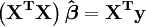
$\sum_{i=1}^{N}\sum_{k=1}^{p} X_{ij}X_{ik}\hat \beta_k=\sum_{i=1}^{N} X_{ij}y_i,\ j=1,p\,$

In matrix notation, the normal equations are written as

$\mathbf{\left(X^TX\right)\hat \boldsymbol \beta=X^Ty}$

For a numerical example see linear regression (example)

Regression diagnostics

Once a regression model has been constructed, it is important to confirm the goodness of fit of the model and the statistical significance of the estimated parameters. Commonly used checks of goodness of fit include the R-squared, analyses of the pattern of residuals and hypothesis testing. Statistical significance is checked by an F-test of the overall fit, followed by t-tests of individual parameters.

Interpretations of these diagnostic tests rest heavily on the model assumptions. Although examination of the residuals can be used to invalidate a model, the results of a t-test or F-test are meaningless unless the modeling assumptions are satisfied.

The error term may not have a normal distribution. See generalized linear model.
The response variable may be non-continuous. For binary (zero or one) variables, there are the probit and logit model. The multivariate probit model makes it possible to estimate jointly the relationship between several binary dependent variables and some independent variables. For categorical variables with more than two values there is the multinomial logit. For ordinal variables with more than two values, there are the ordered logit and ordered probit models. An alternative to such procedures is linear regression based on polychoric or polyserial correlations between the categorical variables. Such procedures differ in the assumptions made about the distribution of the variables in the population. If the variable is positive with low values and represents the repetition of the occurrence of an event, count models like the Poisson regression or the negative binomial model may be used

Interpolation and extrapolation

Regression models predict a value of the $y$ variable given known values of the $x$ variables. If the prediction is to be done within the range of values of the $x$ variables used to construct the model this is known as interpolation. Prediction outside the range of the data used to construct the model is known as extrapolation and it is more risky.

Nonlinear regression

When the model function is not linear in the parameters the sum of squares must be minimized by an iterative procedure. This introduces many complications which are summarized in Differences between linear and non-linear least squares

Other methods

Although the parameters of a regression model are usually estimated using the method of least squares, other methods which have been used include:

Bayesian methods
Minimization of absolute deviations, leading to quantile regression
Nonparametric regression. This approach requires a large number of observations, as the data are used to build the model structure as well as estimate the model parameters. They are usually computationally intensive.

Software

All major statistical software packages perform the common types of regression analysis correctly and in a user-friendly way. Simple linear regression can be done in some spreadsheet applications. There are a number of software programs that perform specialized forms of regression, and experts may choose to write their own code to using statistical programming languages or numerical analysis software.

Retrieved from " http://en.wikipedia.org/w/index.php?title=Regression_analysis&oldid=198424867"