Poisson distribution

Related subjects: Mathematics

Did you know...

SOS Children produced this website for schools as well as this video website about Africa. Click here to find out about child sponsorship.

Poisson
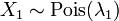
Probability mass function The horizontal axis is the index k. The function is defined only at integer values of k. The connecting lines are only guides for the eye and do not indicate continuity.
Cumulative distribution function The horizontal axis is the index k.
Parameters	$\lambda \in (0,\infty)$
Support	$k \in \{0,1,2,\ldots\}$
PMF	$\frac{e^{-\lambda} \lambda^k}{k!}\!$
CDF	$\frac{\Gamma(\lfloor k+1\rfloor, \lambda)}{\lfloor k\rfloor !}\!\text{ for }k\ge 0$ (where $\Gamma(x, y)$ is the Incomplete gamma function)
Mean	$\lambda\,$
Median	$\text{usually about }\lfloor\lambda+1/3-0.02/\lambda\rfloor$
Mode	$\lfloor\lambda\rfloor$ and $\lambda-1$ if $\lambda$ is an integer
Variance	$\lambda\,$
Skewness	$\lambda^{-1/2}\,$
Ex. kurtosis	$\lambda^{-1}\,$
Entropy	$\lambda[1\!-\!\ln(\lambda)]\!+\!e^{-\lambda}\sum_{k=0}^\infty \frac{\lambda^k\ln(k!)}{k!}$ (for large $\lambda$ ) $\frac{1}{2}\log(2 \pi e \lambda) - \frac{1}{12 \lambda} - \frac{1}{24 \lambda^2} - \frac{19}{360 \lambda^3} + O(\frac{1}{\lambda^4})$
MGF	$\exp(\lambda (e^t-1))\,$
CF	$\exp(\lambda (e^{it}-1))\,$

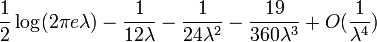
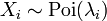
In probability theory and statistics, the Poisson distribution is a discrete probability distribution that expresses the probability of a number of events occurring in a fixed period of time if these events occur with a known average rate and independently of the time since the last event. The Poisson distribution can also be used for the number of events in other specified intervals such as distance, area or volume.

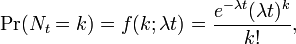
The distribution was discovered by Siméon-Denis Poisson (1781–1840) and published, together with his probability theory, in 1838 in his work Recherches sur la probabilité des jugements en matières criminelles et matière civile ("Research on the Probability of Judgments in Criminal and Civil Matters"). The work focused on certain random variables N that count, among other things, a number of discrete occurrences (sometimes called "arrivals") that take place during a time-interval of given length. If the expected number of occurrences in this interval is λ, then the probability that there are exactly k occurrences (k being a non-negative integer, k = 0, 1, 2, ...) is equal to

$f(k, \lambda)=\frac{\lambda^k e^{-\lambda}}{k!},\,\!$

where

e is the base of the natural logarithm (e = 2.71828...)
k is the number of occurrences of an event - the probability of which is given by the function
k! is the factorial of k
λ is a positive real number, equal to the expected number of occurrences that occur during the given interval. For instance, if the events occur on average every 4 minutes, and you are interested in the number of events occurring in a 10 minute interval, you would use as model a Poisson distribution with λ = 10/4 = 2.5.

As a function of k, this is the probability mass function. The Poisson distribution can be derived as a limiting case of the binomial distribution.

The Poisson distribution can be applied to systems with a large number of possible events, each of which is rare. A classic example is the nuclear decay of atoms.

The Poisson distribution is sometimes called a Poissonian, analogous to the term Gaussian for a Gauss or normal distribution.

Poisson noise and characterizing small occurrences

The parameter λ is not only the mean number of occurrences $\scriptstyle\langle k \rangle$ , but also its variance $\scriptstyle\sigma_k^2 \ \stackrel{\mathrm{def}}{=}\ \langle k^{2} \rangle - \langle k \rangle^{2}$ (see Table). Thus, the number of observed occurrences fluctuates about its mean λ with a standard deviation $\scriptstyle\sigma_{k}\, =\, \sqrt{\lambda}$ . These fluctuations are denoted as Poisson noise or (particularly in electronics) as shot noise.

The correlation of the mean and standard deviation in counting independent, discrete occurrences is useful scientifically. By monitoring how the fluctuations vary with the mean signal, one can estimate the contribution of a single occurrence, even if that contribution is too small to be detected directly. For example, the charge e on an electron can be estimated by correlating the magnitude of an electric current with its shot noise. If N electrons pass a point in a given time t on the average, the mean current is I = eN / t; since the current fluctuations should be of the order $\scriptstyle\sigma_{I} = e\sqrt{N/t\ }$ (i.e. the variance of the Poisson process), the charge e can be estimated from the ratio $\scriptstyle\sigma_{I}^{2}/I$ . An everyday example is the graininess that appears as photographs are enlarged; the graininess is due to Poisson fluctuations in the number of reduced silver grains, not to the individual grains themselves. By correlating the graininess with the degree of enlargement, one can estimate the contribution of an individual grain (which is otherwise too small to be seen unaided). Many other molecular applications of Poisson noise have been developed, e.g., estimating the number density of receptor molecules in a cell membrane.

$\Pr(N_t=k)=f(k;\lambda t)=\frac{e^{-\lambda t} (\lambda t)^k}{k!},\,\!$

Related distributions

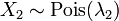If $X_1 \sim \mathrm{Pois}(\lambda_1)\,$ and $X_2 \sim \mathrm{Pois}(\lambda_2)\,$ then the difference $Y = X_1 - X_2$ follows a Skellam distribution.
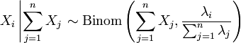
If $X_1 \sim \mathrm{Pois}(\lambda_1)\,$ and $X_2 \sim \mathrm{Pois}(\lambda_2)\,$ are independent, and $Y = X_1 + X_2$ , then the distribution of $X_1$ conditional on $Y=y$ is a binomial. Specifically, $X_1|(Y=y) \sim \mathrm{Binom}(y, \lambda_1/(\lambda_1+\lambda_2))\,$ . More generally, if X₁, X₂,..., X_n are Poisson random variables with parameters λ₁, λ₂,..., λ_n then $X_i \left|\sum_{j=1}^n X_j\right. \sim \mathrm{Binom}\left(\sum_{j=1}^nX_j,\frac{\lambda_i}{\sum_{j=1}^n\lambda_j}\right)$
The Poisson distribution can be derived as a limiting case to the binomial distribution as the number of trials goes to infinity and the expected number of successes remains fixed. Therefore it can be used as an approximation of the binomial distribution if n is sufficiently large and p is sufficiently small. There is a rule of thumb stating that the Poisson distribution is a good approximation of the binomial distribution if n is at least 20 and p is smaller than or equal to 0.05. According to this rule the approximation is excellent if n ≥ 100 and np ≤ 10.
For sufficiently large values of λ, (say λ>1000), the normal distribution with mean λ, and variance λ, is an excellent approximation to the Poisson distribution. If λ is greater than about 10, then the normal distribution is a good approximation if an appropriate continuity correction is performed, i.e., P(X ≤ x), where (lower-case) x is a non-negative integer, is replaced by P(X ≤ x + 0.5).

$F_\mathrm{Poisson}(x;\lambda) \approx F_\mathrm{normal}(x;\mu=\lambda,\sigma^2=\lambda)\,$

If the number of arrivals in a given time follows the Poisson distribution, with mean = $\lambda$ , then the lengths of the inter-arrival times follow the Exponential distribution, with rate $1/\lambda$ .

Occurrence

The Poisson distribution arises in connection with Poisson processes. It applies to various phenomena of discrete nature (that is, those that may happen 0, 1, 2, 3, ... times during a given period of time or in a given area) whenever the probability of the phenomenon happening is constant in time or space. Examples of events that may be modelled as a Poisson distribution include:

The number of cars that pass through a certain point on a road (sufficiently distant from traffic lights) during a given period of time.
The number of spelling mistakes one makes while typing a single page.
The number of phone calls at a call centre per minute.
The number of times a web server is accessed per minute.
The number of roadkill (animals killed) found per unit length of road.
The number of mutations in a given stretch of DNA after a certain amount of radiation.
The number of unstable nuclei that decayed within a given period of time in a piece of radioactive substance. The radioactivity of the substance will weaken with time, so the total time interval used in the model should be significantly less than the mean lifetime of the substance.
The number of pine trees per unit area of mixed forest.
The number of stars in a given volume of space.
The number of soldiers killed by horse-kicks each year in each corps in the Prussian cavalry. This example was made famous by a book of Ladislaus Josephovich Bortkiewicz (1868–1931).
The distribution of visual receptor cells in the retina of the human eye.
The number of light bulbs that burn out in a certain amount of time.
The number of viruses that can infect a cell in cell culture.
The number of hematopoietic stem cells in a sample of unfractionated bone marrow cells.
The number of inventions of an inventor over their career.
The number of particles that "scatter" off of a target in a nuclear or high energy physics experiment.

[Note: the intervals between successive Poisson events are reciprocally-related, following the Exponential distribution. For example, the lifetime of a lightbulb, or waiting time between buses.]

How does this distribution arise? — The law of rare events

In several of the above examples—for example, the number of mutations in a given sequence of DNA—the events being counted are actually the outcomes of discrete trials, and would more precisely be modelled using the binomial distribution. However, the binomial distribution with parameters n and λ/n, i.e., the probability distribution of the number of successes in n trials, with probability λ/n of success on each trial, approaches the Poisson distribution with expected value λ as n approaches infinity. This limit is sometimes known as the law of rare events, although this name may be misleading because the events in a Poisson process need not be rare (the number of telephone calls to a busy switchboard in one hour follows a Poisson distribution, but these events would not be considered rare). It provides a means by which to approximate random variables using the Poisson distribution rather than the more-cumbersome binomial distribution.

Here are the details. First, recall from calculus that

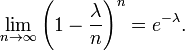
$\lim_{n\to\infty}\left(1-{\lambda \over n}\right)^n=e^{-\lambda}.$

Let p = λ/n. Then we have

$\lim_{n\to\infty} \Pr(X=k)=\lim_{n\to\infty}{n \choose k} p^k (1-p)^{n-k} =\lim_{n\to\infty}{n! \over (n-k)!k!} \left({\lambda \over n}\right)^k \left(1-{\lambda\over n}\right)^{n-k}$

$=\lim_{n\to\infty} \underbrace{\left({n \over n}\right)\left({n-1 \over n}\right)\left({n-2 \over n}\right) \cdots \left({n-k+1 \over n}\right)}\ \underbrace{\left({\lambda^k \over k!}\right)}\ \underbrace{\left(1-{\lambda \over n}\right)^n}\ \underbrace{\left(1-{\lambda \over n}\right)^{-k}}$

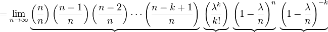
As n approaches ∞, the expression over the first underbrace approaches 1; the second remains constant since "n" does not appear in it at all; the third approaches e^−λ; and the fourth expression approaches 1.

Consequently the limit is

${\lambda^k e^{-\lambda} \over k!}.\,\!$

More generally, whenever a sequence of binomial random variables with parameters n and p_n is such that

$\lim_{n\rightarrow\infty} np_n = \lambda,$

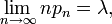
the sequence converges in distribution to a Poisson random variable with mean λ (see, e.g. law of rare events).

Properties

The expected value of a Poisson-distributed random variable is equal to λ and so is its variance. The higher moments of the Poisson distribution are Touchard polynomials in λ, whose coefficients have a combinatorial meaning. In fact when the expected value of the Poisson distribution is 1, then Dobinski's formula says that the nth moment equals the number of partitions of a set of size n.

The mode of a Poisson-distributed random variable with non-integer λ is equal to $\scriptstyle\lfloor \lambda \rfloor$ , which is the largest integer less than or equal to λ. This is also written as floor(λ). When λ is a positive integer, the modes are λ and λ − 1.

Sums of Poisson-distributed random variables:

If $X_i \sim \mathrm{Poi}(\lambda_i)\,$ follow a Poisson distribution with parameter $\lambda_i\,$ and $X_i$ are independent, then 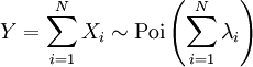$Y = \sum_{i=1}^N X_i \sim \mathrm{Poi}\left(\sum_{i=1}^N \lambda_i\right)\,$ also follows a Poisson distribution whose parameter is the sum of the component parameters.

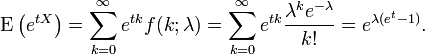
The moment-generating function of the Poisson distribution with expected value λ is

$\mathrm{E}\left(e^{tX}\right)=\sum_{k=0}^\infty e^{tk} f(k;\lambda)=\sum_{k=0}^\infty e^{tk} {\lambda^k e^{-\lambda} \over k!} =e^{\lambda(e^t-1)}.$

All of the cumulants of the Poisson distribution are equal to the expected value λ. The nth factorial moment of the Poisson distribution is λⁿ.

The Poisson distributions are infinitely divisible probability distributions.

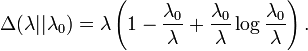
The directed Kullback-Leibler divergence between Poi(λ₀) and Poi(λ) is given by

$\Delta(\lambda||\lambda_0) = \lambda \left( 1 - \frac{\lambda_0}{\lambda} + \frac{\lambda_0}{\lambda} \log \frac{\lambda_0}{\lambda} \right).$

Generating Poisson-distributed random variables

A simple way to generate random Poisson-distributed numbers is given by Knuth, see References below.

algorithm poisson random number (Knuth):
    init:
         Let L ← e^−λ, k ← 0 and p ← 1.
    do:
         k ← k + 1.
         Generate uniform random number u in [0,1] and let p ← p × u.
    while p ≥ L.
    return k − 1.

While simple, the complexity is linear in λ. There are many other algorithms to overcome this. Some are given in Ahrens & Dieter, see References below.

Parameter estimation

Maximum likelihood

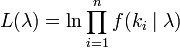
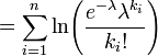
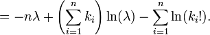
Given a sample of n measured values k_i we wish to estimate the value of the parameter λ of the Poisson population from which the sample was drawn. To calculate the maximum likelihood value, we form the log-likelihood function

$L(\lambda) = \ln \prod_{i=1}^n f(k_i \mid \lambda) \!$

$= \sum_{i=1}^n \ln\!\left(\frac{e^{-\lambda}\lambda^{k_i}}{k_i!}\right) \!$

$= -n\lambda + \left(\sum_{i=1}^n k_i\right) \ln(\lambda) - \sum_{i=1}^n \ln(k_i!). \!$

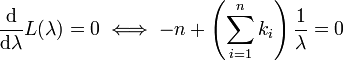
Take the derivative of L with respect to λ and equate it to zero:

$\frac{\mathrm{d}}{\mathrm{d}\lambda} L(\lambda) = 0 \iff -n + \left(\sum_{i=1}^n k_i\right) \frac{1}{\lambda} = 0 \!$

Solving for λ yields the maximum-likelihood estimate of λ:

$\widehat{\lambda}_\mathrm{MLE}=\frac{1}{n}\sum_{i=1}^n k_i. \!$

Since each observation has expectation λ so does this sample mean. Therefore it is an unbiased estimator of λ. It is also an efficient estimator, i.e. its estimation variance achieves the Cramér-Rao lower bound (CRLB).

Bayesian inference

In Bayesian inference, the conjugate prior for the rate parameter λ of the Poisson distribution is the Gamma distribution. Let

$\lambda \sim \mathrm{Gamma}(\alpha, \beta) \!$

denote that λ is distributed according to the Gamma density g parameterized in terms of a shape parameter α and an inverse scale parameter β:

$g(\lambda \mid \alpha,\beta) = \frac{\beta^{\alpha}}{\Gamma(\alpha)} \; \lambda^{\alpha-1} \; e^{-\beta\,\lambda} \qquad \mbox{for}\ \lambda>0 \,\!.$

Then, given the same sample of n measured values k_i as before, and a prior of Gamma(α, β), the posterior distribution is

$\lambda \sim \mathrm{Gamma}(\alpha + \sum_{i=1}^n k_i, \frac{1}{\frac{1}{\beta} + n}). \!$

The posterior mean E[λ] approaches the maximum likelihood estimate $\widehat{\lambda}_\mathrm{MLE}$ in the limit as $\alpha\to 0,\ \beta\to 0$ .

The posterior predictive distribution of additional data is a Gamma-Poisson (i.e. negative binomial) distribution.

The "law of small numbers"

The word law is sometimes used as a synonym of probability distribution, and convergence in law means convergence in distribution. Accordingly, the Poisson distribution is sometimes called the law of small numbers because it is the probability distribution of the number of occurrences of an event that happens rarely but has very many opportunities to happen. The Law of Small Numbers is a book by Ladislaus Bortkiewicz about the Poisson distribution, published in 1898. Some historians of mathematics have argued that the Poisson distribution should have been called the Bortkiewicz distribution.

Calculating an approximation of the Poisson probability

When k becomes large (>20) the use of logs and factorial approximations are needed. Here is an example written in Java.

/**Calculates an approximation of the Poisson probability.
 * @param mean - lambda, the average number of occurrences
 * @param observed - the actual number of occurences observed
 * @return ln(Poisson probability) - the natural log of the Poisson probability.
 */
public static double poissonProbabilityApproximation (double mean, int observed) {
        double k = observed;
        double a = k * Math.log(mean);
        double b = -mean;
        return a + b - factorialApproximation(k);
}
 
/**Srinivasa Ramanujan ln(n!) factorial estimation.
 * Good for larger values of n.
 * @return ln(n!)
 */
public static double factorialApproximation(double n) {
        if (n < 2.) return 0;
        double a = n * Math.log(n) - n;
        double b = Math.log(n * (1. + 4. * n * (1. + 2. * n))) / 6.;
        return a + b + Math.log(Math.PI) / 2.;
}

Online Visualization Tools

SOCR distribution GUI
TAMU's Interactive Poisson Distribution

Retrieved from " http://en.wikipedia.org/w/index.php?title=Poisson_distribution&oldid=197206369"