
Lebesgue integration
Background to the schools Wikipedia
SOS believes education gives a better chance in life to children in the developing world too. Click here to find out about child sponsorship.

In mathematics, the integral of a non-negative function can be regarded in the simplest case as the area between the graph of that function and the x-axis. Lebesgue integration is a mathematical construction that extends the integral to a larger class of functions; it also extends the domains on which these functions can be defined. It had long been understood that for non-negative functions with a smooth enough graph (such as continuous functions on closed bounded intervals) the area under the curve could be defined as the integral and computed using techniques of approximation of the region by polygons. However, as the need to consider more irregular functions arose (for example, as a result of the limiting processes of mathematical analysis and the mathematical theory of probability) it became clear that more careful approximation techniques would be needed to define a suitable integral. Also, we might wish to integrate on spaces more general than the real line; the Lebesgue integral provides the right abstractions needed to do this important job.
The Lebesgue integral plays an important role in the branch of mathematics called real analysis and in many other fields in the mathematical sciences, and is named after Henri Lebesgue (1875–1941) who introduced the integral in (Lebesgue 1904). It is also a pivotal portion of the axiomatic theory of probability.
The term "Lebesgue integration" may refer either to the general theory of integration of a function with respect to a general measure, as introduced by Lebesgue, or to the specific case of integration of a function defined on a sub-domain of the real line with respect to Lebesgue measure.
Introduction
The integral of a function f between limits a and b can be interpreted as the area under the graph of f. This is easy to understand for familiar functions such as polynomials, but what does it mean for more exotic functions? In general, what is the class of functions for which "area under the curve" makes sense? The answer to this question has great theoretical and practical importance.
As part of a general movement toward rigour in mathematics in the nineteenth century, attempts were made to put the integral calculus on a firm foundation. The Riemann integral, proposed by Bernhard Riemann (1826–1866), is a broadly successful attempt to provide such a foundation. Riemann's definition starts with the construction of a sequence of easily-calculated areas which converge to the integral of a given function. This definition is successful in the sense that it gives the expected answer for many already-solved problems, and gives useful results for many other problems.
However, Riemann integration does not interact well with taking limits of sequences of functions, making such limiting processes difficult to analyze. This is of prime importance, for instance, in the study of Fourier series, Fourier transforms and other topics. The Lebesgue integral is better able to describe how and when it is possible to take limits under the integral sign. The Lebesgue definition considers a different class of easily-calculated areas than the Riemann definition, which is the main reason the Lebesgue integral is better behaved. The Lebesgue definition also makes it possible to calculate integrals for a broader class of functions. For example, the Dirichlet function, which is 0 where its argument is irrational and 1 otherwise, has a Lebesgue integral, but it does not have a Riemann integral.
Lebesgue's approach to integration was summarized in a letter to Paul Montel. He writes:
I have to pay a certain sum, which I have collected in my pocket. I take the bills and coins out of my pocket and give them to the creditor in the order I find them until I have reached the total sum. This is the Riemann integral. But I can proceed differently. After I have taken all the money out of my pocket I order the bills and coins according to identical values and then I pay the several heaps one after the other to the creditor. This is my integral.—Source: (Siegmund-Schultze 2008)
The insight is that one should be able to rearrange the values of a function freely while preserving the value of the integral. This process of rearrangement can convert a very pathological function into one which is "nice" from the point of view of integration, and thus allows for such pathological functions to be integrated.
Intuitive interpretation

To get some intuition about the different approaches to integration, let us imagine that it is desired to find a mountain's volume (above sea level).
- The Riemann-Darboux approach
- Divide the base of the mountain into a grid of 1 meter squares. Measure the altitude of the mountain at the centre of each square. The volume on a single grid square is approximately 1×1×(altitude), so the total volume is the sum of the altitudes.
- The Lebesgue approach
- Draw a contour map of the mountain, where adjacent contours are 1 meter of altitude apart. The volume of earth contained in a single contour is approximately that contour's area times 1, so the total volume is the sum of these areas times 1 meter.
Folland summarizes the difference between the Riemann and Lebesgue approaches thus: "to compute the Riemann integral of f, one partitions the domain [a, b] into subintervals", while in the Lebesgue integral, "one is in effect partitioning the range of f".
Toward a formal definition
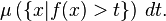
To define the Lebesgue integral formally requires the notion of a measure which, roughly, associates to each set A of real numbers a nonnegative number μ(A) representing the "size" of A. This notion of "size" should agree with the usual length of an interval or disjoint union of intervals. Suppose that f : R → R is a non-negative real-valued function. Using the "partitioning the range of f" philosophy, the integral of f should be the sum over t of the areas between a thin horizontal strip between y = t and y = t+dt. This area is just
Let

The Lebesgue integral of f is then defined by
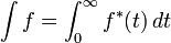
where the integral on the right is an ordinary improper Riemann integral (note that f* is a strictly decreasing positive function, and therefore has a well-defined improper Riemann integral). For a suitable class of functions (the measurable functions) this defines the Lebesgue integral.
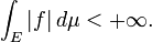
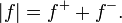
A general (not necessarily positive) function f is Lebesgue integrable if the area between the graph of f and the x-axis is finite:
In that case, the integral is, as in the Riemannian case, the difference between the area above the x-axis and the area below the x-axis:
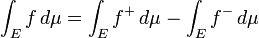
where
Construction

The discussion that follows parallels the most common expository approach to the Lebesgue integral. In this approach, the theory of integration has two distinct parts:
- A theory of measurable sets and measures on these sets.
- A theory of measurable functions and integrals on these functions.
The function whose integral is to be found is then approximated by certain so-called simple functions, whose integrals can be written in terms of the measure. The integral of the original function is then the limit of the integral of the simple functions.
Measure theory
Measure theory was initially created to provide a useful abstraction of the notion of length of subsets of the real line and, more generally, area and volume of subsets of Euclidean spaces. In particular, it provided a systematic answer to the question of which subsets of R have a length. As was shown by later developments in set theory (see non-measurable set), it is actually impossible to assign a length to all subsets of R in a way which preserves some natural additivity and translation invariance properties. This suggests that picking out a suitable class of measurable subsets is an essential prerequisite.
The Riemann integral uses the notion of length explicitly. Indeed, the element of calculation for the Riemann integral is the rectangle [a, b] × [c, d], whose area is calculated to be (b − a)(d − c). The quantity b − a is the length of the base of the rectangle and d − c is the height of the rectangle. Riemann could only use planar rectangles to approximate the area under the curve because there was no adequate theory for measuring more general sets.
In the development of the theory in most modern textbooks (after 1950), the approach to measure and integration is axiomatic. This means that a measure is any function μ defined on a certain class X of subsets of a set E, which satisfies a certain list of properties. These properties can be shown to hold in many different cases.
Integration
We start with a measure space (E, X, μ) where E is a set, X is a σ-algebra of subsets of E and μ is a (non- negative) measure on E, defined on the sets of X.
For example, E can be Euclidean n-space Rn or some Lebesgue measurable subset of it, X will be the σ-algebra of all Lebesgue measurable subsets of E, and μ will be the Lebesgue measure. In the mathematical theory of probability, we confine our study to a probability measure μ, which satisfies μ(E) = 1.
In Lebesgue's theory, integrals are defined for a class of functions called measurable functions. A function f is measurable if the pre-image of every interval of the form (t, ∞) is in X:

It can be shown that this is equivalent to requiring that the pre-image of any Borel subset of R be in X. We will make this assumption henceforth. The set of measurable functions is closed under algebraic operations, but more importantly the class is closed under various kinds of pointwise sequential limits:
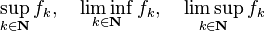
are measurable if the original sequence (fk)k, where k ∈ N, consists of measurable functions.
We build up an integral
for measurable real-valued functions f defined on E in stages:
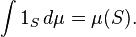
Indicator functions: To assign a value to the integral of the indicator function 1S of a measurable set S consistent with the given measure μ, the only reasonable choice is to set:
Notice that the result may be equal to +∞, unless μ is a finite measure.
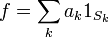
Simple functions: A finite linear combination of indicator functions

where the coefficients ak are real numbers and the sets Sk are measurable, is called a measurable simple function. We extend the integral by linearity to non-negative measurable simple functions. When the coefficients ak are non-negative, we set
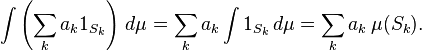
The convention 0 × ∞ = 0 must be used, and the result may be infinite. Even if a simple function can be written in many ways as a linear combination of indicator functions, the integral will always be the same; this can be shown using the additivity property of measures.
Some care is needed when defining the integral of a real-valued simple function, to avoid the undefined expression ∞ − ∞: one assumes that the representation
is such that μ(Sk) < ∞ whenever ak ≠ 0. Then the above formula for the integral of f makes sense, and the result does not depend upon the particular representation of f satisfying the assumptions.
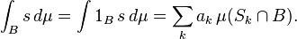
If B is a measurable subset of E and s is a measurable simple function one defines
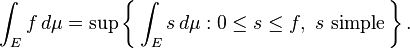
Non-negative functions: Let f be a non-negative measurable function on E which we allow to attain the value +∞, in other words, f takes non-negative values in the extended real number line. We define
We need to show this integral coincides with the preceding one, defined on the set of simple functions. When E is a segment [a, b], there is also the question of whether this corresponds in any way to a Riemann notion of integration. It is possible to prove that the answer to both questions is yes.
We have defined the integral of f for any non-negative extended real-valued measurable function on E. For some functions, this integral ∫E f dμ will be infinite.
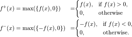
Signed functions: To handle signed functions, we need a few more definitions. If f is a measurable function of the set E to the reals (including ±∞), then we can write
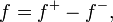
where
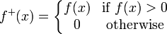
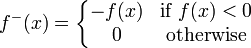
Note that both f+ and f− are non-negative measurable functions. Also note that
We say that the Lebesgue integral of the measurable function f exists, or is defined if at least one of  and
and  is finite:
In this case we define
If
we say that f is Lebesgue integrable.
It turns out that this definition gives the desirable properties of the integral.
Complex valued functions can be similarly integrated, by considering the real part and the imaginary part separately.
Example
Consider the indicator function of the rational numbers, 1Q. This function is nowhere continuous.
 is not Riemann-integrable on [0,1]: No matter how the set [0,1] is partitioned into subintervals, each partition will contain at least one rational and at least one irrational number, because rationals and irrationals are both dense in the reals. Thus the upper Darboux sums will all be one, and the lower Darboux sums will all be zero.
- is Lebesgue-integrable on [0,1] using the Lebesgue measure: Indeed it is the indicator function of the rationals so by definition
![\int_{[0,1]} 1_{\mathbf Q} \, d \mu = \mu(\mathbf{Q} \cap [0,1]) = 0,](../../images/2452/245211.png)
- because Q is countable.
Domain of integration
A technical issue in Lebesgue integration is that the domain of integration is defined as a set (a subset of a measure space), with no notion of orientation. In elementary calculus, one defines integration with respect to an orientation:
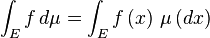
Generalizing this to higher dimensions yields integration of differential forms. By contrast, Lebesgue integration provides an alternative generalization, integrating over subsets with respect to a measure; this can be notated as
![\int_A f\,d\mu = \int_{[a,b]} f\,d\mu](../../images/2452/245213.png)
to indicate integration over a subset A. For details on the relation between these generalizations, see Differential form: Relation with measures.
Limitations of the Riemann integral
Here we discuss the limitations of the Riemann integral and the greater scope offered by the Lebesgue integral. We presume a working understanding of the Riemann integral.
With the advent of Fourier series, many analytical problems involving integrals came up whose satisfactory solution required interchanging limit processes and integral signs. However, the conditions under which the integrals
![\sum_k \int f_k(x) dx, \quad \int \left [\sum_k f_k(x) \right ] dx](../../images/2452/245214.png)
are equal proved quite elusive in the Riemann framework. There are some other technical difficulties with the Riemann integral. These are linked with the limit-taking difficulty discussed above.
Failure of monotone convergence. As shown above, the indicator function 1Q on the rationals is not Riemann integrable. In particular, the Monotone convergence theorem fails. To see why, let {ak} be an enumeration of all the rational numbers in [0,1] (they are countable so this can be done.) Then let
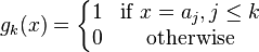
The function gk is zero everywhere except on a finite set of points, hence its Riemann integral is zero. The sequence gk is also clearly non-negative and monotonically increasing to 1Q, which is not Riemann integrable.
Unsuitability for unbounded intervals. The Riemann integral can only integrate functions on a bounded interval. It can however be extended to unbounded intervals by taking limits, so long as this doesn't yield an answer such as ∞−∞.
Integrating on structures other than Euclidean space. The Riemann integral is inextricably linked to the order structure of the line.
Basic theorems of the Lebesgue integral
The Lebesgue integral does not distinguish between functions which differ only on a set of μ-measure zero. To make this precise, functions f and g are said to be equal almost everywhere (a.e.) if

- If f, g are non-negative measurable functions (possibly assuming the value +∞) such that f = g almost everywhere, then
To wit, the integral respects the equivalence relation of almost-everywhere equality.
- If f, g are functions such that f = g almost everywhere, then f is Lebesgue integrable if and only if g is Lebesgue integrable, and the integrals of f and g are the same if they exist.
The Lebesgue integral has the following properties:
Linearity: If f and g are Lebesgue integrable functions and a and b are real numbers, then af + bg is Lebesgue integrable and
Monotonicity: If f ≤ g, then
Monotone convergence theorem: Suppose {fk}k ∈ N is a sequence of non-negative measurable functions such that

Then, the pointwise limit f of fk is Lebesgue integrable and
Note: The value of any of the integrals is allowed to be infinite.
Fatou's lemma: If {fk}k ∈ N is a sequence of non-negative measurable functions, then
Again, the value of any of the integrals may be infinite.
Dominated convergence theorem: Suppose {fk}k ∈ N is a sequence of complex measurable functions with pointwise limit f, and there is a Lebesgue integrable function g (i.e., g belongs to the space L1) such that |fk| ≤ g for all k.
Then, f is Lebesgue integrable and
Proof techniques
To illustrate some of the proof techniques used in Lebesgue integration theory, we sketch a proof of the above mentioned Lebesgue monotone convergence theorem. Let {fk}k ∈ N be a non-decreasing sequence of non-negative measurable functions and put
By the monotonicity property of the integral, it is immediate that:
and the limit on the right exists, because the sequence is monotonic. We now prove the inequality in the other direction. It follows from the definition of integral that there is a non-decreasing sequence (gn) of non-negative simple functions such that gn ≤ f and
Therefore, it suffices to prove that for each n ∈ N,
We will show that if g is a simple function and
almost everywhere, then
By breaking up the function g into its constant value parts, this reduces to the case in which g is the indicator function of a set. The result we have to prove is then
Suppose A is a measurable set and {fk}k ∈ N is a nondecreasing sequence of non-negative measurable functions on E such that
for almost all x ∈ A. Then
To prove this result, fix ε > 0 and define the sequence of measurable sets

By monotonicity of the integral, it follows that for any k ∈ N,
Because almost every x will be in Bk for large enough k, we have

up to a set of measure 0. Thus by countable additivity of μ, and because Bk increases with k,
As this is true for any positive ε the result follows.
Alternative formulations
It is possible to develop the integral with respect to the Lebesgue measure without relying on the full machinery of measure theory. One such approach is provided by the Daniell integral.
There is also an alternative approach to developing the theory of integration via methods of functional analysis. The Riemann integral exists for any continuous function f of compact support defined on Rn (or a fixed open subset). Integrals of more general functions can be built starting from these integrals.
Let Cc be the space of all real-valued compactly supported continuous functions of R. Define a norm on Cc by
Then Cc is a normed vector space (and in particular, it is a metric space.) All metric spaces have Hausdorff completions, so let L1 be its completion. This space is isomorphic to the space of Lebesgue integrable functions modulo the subspace of functions with integral zero. Furthermore, the Riemann integral ∫ is a uniformly continuous functional with respect to the norm on Cc, which is dense in L1. Hence ∫ has a unique extension to all of L1. This integral is precisely the Lebesgue integral.
More generally, when the measure space on which the functions are defined is also a locally compact topological space (as is the case with the real numbers R), measures compatible with the topology in a suitable sense ( Radon measures, of which the Lebesgue measure is an example) an integral with respect to them can be defined in the same manner, starting from the integrals of continuous functions with compact support. More precisely, the compactly supported functions form a vector space that carries a natural topology, and a (Radon) measure is defined as a continuous linear functional on this space. The value of a measure at a compactly supported function is then also by definition the integral of the function. One then proceeds to expand the measure (the integral) to more general functions by continuity, and defines the measure of a set as the integral of its indicator function. This is the approach taken by Bourbaki (2004) and a certain number of other authors. For details see Radon measures.
Limitations of Lebesgue integral
The main purpose of Lebesgue integral is to provide an integral notation where limits of integrals hold under mild assumptions. There is no guarantee that every function is Lebesgue integrable. It may happen that improper (Riemann) integrals exist for functions that are not Lebesgue integrable. One example would be

This function is not Lebesgue integrable as
On the other hand, it exists as an improper Riemann integral and the integral can be computed to be finite. An equivalent concept of improper Lebesgue integral does not exist because such a perspective is unnecessary from the viewpoint of the convergence theorems.